How Do You Know You Have a Standing Wave in a Tube

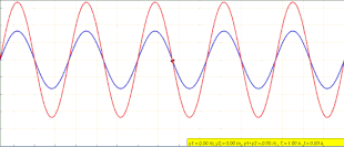
Blitheness of a standing wave (red) created by the superposition of a left traveling (blueish) and right traveling (greenish) wave

Longitudinal continuing wave

In physics, a standing wave, as well known as a stationary moving ridge, is a wave that oscillates in time but whose summit amplitude profile does not move in space. The superlative amplitude of the wave oscillations at any point in space is abiding with respect to fourth dimension, and the oscillations at different points throughout the moving ridge are in phase. The locations at which the absolute value of the aamplitude is minimum are called nodes, and the locations where the absolute value of the amplitude is maximum are called antinodes.

Continuing waves were first noticed by Michael Faraday in 1831. Faraday observed standing waves on the surface of a liquid in a vibrating container.^{[one] [ii]} Franz Melde coined the term "standing wave" (High german: stehende Welle or Stehwelle) around 1860 and demonstrated the phenomenon in his classic experiment with vibrating strings.^{[3] [four] [5] [six]}

This phenomenon can occur considering the medium is moving in the management opposite to the move of the wave, or it tin can arise in a stationary medium every bit a consequence of interference between ii waves traveling in opposite directions. The well-nigh mutual cause of standing waves is the phenomenon of resonance, in which standing waves occur inside a resonator due to interference between waves reflected back and forth at the resonator's resonant frequency.

For waves of equal amplitude traveling in opposing directions, there is on boilerplate no net propagation of energy.

Moving medium [edit]

Every bit an instance of the outset type, under certain meteorological conditions standing waves grade in the atmosphere in the lee of mountain ranges. Such waves are frequently exploited past glider pilots.

Standing waves and hydraulic jumps as well grade on fast flowing river rapids and tidal currents such as the Saltstraumen maelstrom. A requirement for this in river currents is a flowing h2o with shallow depth in which the inertia of the water overcomes its gravity due to the supercritical flow speed (Froude number: one.7 - 4.5, surpassing iv.five results in straight standing wave^[7]) and is therefore neither significantly slowed downwardly by the obstacle nor pushed to the side. Many standing river waves are popular river surfing breaks.

Opposing waves [edit]

Standing waves

Standing wave in stationary medium. The cerise dots represent the wave nodes. A standing wave (black) depicted equally the sum of 2 propagating waves traveling in opposite directions (red and blueish).

Electrical forcefulness vector (E) and magnetic force vector (H) of a continuing wave.

As an example of the 2nd type, a standing wave in a transmission line is a wave in which the distribution of current, voltage, or field strength is formed by the superposition of two waves of the same frequency propagating in opposite directions. The upshot is a serial of nodes (zero displacement) and anti-nodes (maximum displacement) at fixed points forth the transmission line. Such a standing wave may exist formed when a wave is transmitted into one end of a transmission line and is reflected from the other end by an impedance mismatch, i.e., aperture, such every bit an open circuit or a short.^[viii] The failure of the line to transfer power at the continuing moving ridge frequency volition usually result in attenuation distortion.

In practice, losses in the manual line and other components mean that a perfect reflection and a pure standing moving ridge are never achieved. The result is a fractional standing moving ridge, which is a superposition of a continuing wave and a traveling wave. The caste to which the wave resembles either a pure standing wave or a pure traveling moving ridge is measured past the standing moving ridge ratio (SWR).^[9]

Another instance is standing waves in the open body of water formed by waves with the aforementioned wave catamenia moving in contrary directions. These may grade near storm centres, or from reflection of a smashing at the shore, and are the source of microbaroms and microseisms.

Mathematical description [edit]

This section considers representative one- and two-dimensional cases of continuing waves. Offset, an example of an space length string shows how identical waves traveling in opposite directions interfere to produce standing waves. Side by side, ii finite length cord examples with different boundary conditions demonstrate how the purlieus conditions restrict the frequencies that can course continuing waves. Next, the example of audio waves in a pipe demonstrates how the same principles can exist applied to longitudinal waves with analogous purlieus conditions.

Continuing waves tin can likewise occur in ii- or three-dimensional resonators. With standing waves on ii-dimensional membranes such as drumheads, illustrated in the animations higher up, the nodes become nodal lines, lines on the surface at which there is no move, that separate regions vibrating with reverse phase. These nodal line patterns are called Chladni figures. In 3-dimensional resonators, such equally musical instrument sound boxes and microwave cavity resonators, there are nodal surfaces. This department includes a two-dimensional standing wave example with a rectangular boundary to illustrate how to extend the concept to college dimensions.

Continuing wave on an infinite length string [edit]

To begin, consider a string of infinite length along the x-centrality that is complimentary to exist stretched transversely in the y management.

For a harmonic moving ridge traveling to the correct along the string, the string'south displacement in the y direction as a function of position x and time t is^[10]

${\displaystyle y_{\text{R}}(x,t)=y_{\text{max}}\sin \left({2\pi x \over \lambda }-\omega t\right).}$

The displacement in the y-direction for an identical harmonic wave traveling to the left is

${\displaystyle y_{\text{L}}(x,t)=y_{\text{max}}\sin \left({2\pi x \over \lambda }+\omega t\right),}$

where

• y _max is the aamplitude of the deportation of the string for each moving ridge,
• ω is the angular frequency or equivalently 2π times the frequency f,
• λ is the wavelength of the wave.

For identical correct- and left-traveling waves on the same string, the total displacement of the string is the sum of y _R and y ₅₀,

${\displaystyle y(x,t)=y_{\text{R}}+y_{\text{L}}=y_{\text{max}}\sin \left({two\pi x \over \lambda }-\omega t\right)+y_{\text{max}}\sin \left({2\pi x \over \lambda }+\omega t\right).}$

Using the trigonometric sum-to-production identity ${\displaystyle \sin a+\sin b=2\sin \left({a+b \over 2}\right)\cos \left({a-b \over two}\right)}$ ,

${\displaystyle y(x,t)=2y_{\text{max}}\sin \left({2\pi x \over \lambda }\right)\cos(\omega t).}$

(one)

Annotation that Equation (1) does not describe a traveling wave. At any position x, y(10,t) just oscillates in time with an aamplitude that varies in the 10-direction as ${\displaystyle 2y_{\text{max}}\sin \left({2\pi ten \over \lambda }\correct)}$ .^[10] The animation at the beginning of this article depicts what is happening. As the left-traveling blue wave and right-traveling green wave interfere, they form the standing red wave that does not travel and instead oscillates in place.

Because the string is of space length, information technology has no purlieus status for its displacement at any point along the x-axis. Equally a consequence, a standing wave can course at any frequency.

At locations on the x-axis that are even multiples of a quarter wavelength,

${\displaystyle x=\ldots ,-{3\lambda \over ii},\;-\lambda ,\;-{\lambda \over 2},\;0,\;{\lambda \over 2},\;\lambda ,\;{3\lambda \over two},\ldots }$

the amplitude is always zero. These locations are called nodes. At locations on the x-axis that are odd multiples of a quarter wavelength

${\displaystyle ten=\ldots ,-{5\lambda \over 4},\;-{3\lambda \over 4},\;-{\lambda \over 4},\;{\lambda \over iv},\;{3\lambda \over four},\;{5\lambda \over 4},\ldots }$

the aamplitude is maximal, with a value of twice the amplitude of the correct- and left-traveling waves that interfere to produce this standing wave pattern. These locations are called anti-nodes. The distance between two consecutive nodes or anti-nodes is one-half the wavelength, λ/2.

Standing wave on a cord with 2 stock-still ends [edit]

Adjacent, consider a string with fixed ends at 10 = 0 and x = L . The string will accept some damping as information technology is stretched by traveling waves, but presume the damping is very pocket-sized. Suppose that at the x = 0 fixed finish a sinusoidal force is applied that drives the cord upward and down in the y-direction with a small amplitude at some frequency f. In this situation, the driving force produces a right-traveling wave. That moving ridge reflects off the right fixed end and travels dorsum to the left, reflects once again off the left fixed finish and travels dorsum to the right, and so on. Somewhen, a steady land is reached where the string has identical correct- and left-traveling waves as in the infinite-length case and the ability dissipated by damping in the cord equals the power supplied by the driving force so the waves have constant amplitude.

Equation (1) notwithstanding describes the standing wave pattern that can course on this string, but now Equation (1) is subject to boundary conditions where y = 0 at 10 = 0 and x = Fifty because the cord is stock-still at x = L and considering we assume the driving force at the fixed 10 = 0 finish has small amplitude. Checking the values of y at the ii ends,

${\displaystyle y(0,t)=0,}$

${\displaystyle y(L,t)=2y_{\text{max}}\sin \left({2\pi L \over \lambda }\right)\cos(\omega t)=0.}$

This purlieus condition is in the form of the Sturm–Liouville formulation. The latter boundary condition is satisfied when ${\displaystyle \sin \left({ii\pi 50 \over \lambda }\correct)=0}$ . L is given, so the boundary condition restricts the wavelength of the standing waves to^[11]

${\displaystyle \lambda ={\frac {2L}{n}},}$

(2)

${\displaystyle n=1,2,three,\ldots }$

Waves can only form continuing waves on this string if they take a wavelength that satisfies this relationship with L. If waves travel with speed v forth the cord, and so equivalently the frequency of the standing waves is restricted to^{[11] [12]}

${\displaystyle f={\frac {v}{\lambda }}={\frac {nv}{2L}}.}$

The standing wave with n = ane oscillates at the fundamental frequency and has a wavelength that is twice the length of the cord. Higher integer values of n correspond to modes of oscillation chosen harmonics or overtones. Any standing wave on the cord volition have n + one nodes including the fixed ends and n anti-nodes.

To compare this case's nodes to the description of nodes for standing waves in the infinite length string, note that Equation (2) can be rewritten as

${\displaystyle \lambda ={\frac {4L}{northward}},}$

${\displaystyle north=ii,iv,six,\ldots }$

In this variation of the expression for the wavelength, n must exist even. Cross multiplying we see that because L is a node, it is an even multiple of a quarter wavelength,

${\displaystyle L={\frac {n\lambda }{4}},}$

${\displaystyle n=ii,4,6,\ldots }$

This example demonstrates a type of resonance and the frequencies that produce continuing waves can exist referred to as resonant frequencies.^{[11] [thirteen] [14]}

Standing wave on a string with ane fixed end [edit]

Adjacent, consider the same string of length L, but this time information technology is only fixed at x = 0. At x = L , the cord is free to move in the y management. For instance, the cord might be tied at 10 = Fifty to a ring that can slide freely upward and downwardly a pole. The cord once again has small damping and is driven past a small-scale driving force at ten = 0.

In this instance, Equation (one) withal describes the standing wave pattern that can course on the string, and the cord has the aforementioned boundary status of y = 0 at x = 0. However, at ten = L where the cord can move freely in that location should be an anti-node with maximal amplitude of y. Equivalently, this boundary status of the "free end" can exist stated as ∂y/∂x = 0 at x = L , which is in the form of the Sturm–Liouville formulation. The intuition for this boundary status ∂y/∂ten = 0 at x = Fifty is that the motion of the "gratis cease" volition follow that of the indicate to its left.

Reviewing Equation (1), for x = L the largest amplitude of y occurs when ∂y/∂10 = 0, or

${\displaystyle \cos \left({ii\pi L \over \lambda }\right)=0.}$

This leads to a dissimilar set of wavelengths than in the 2-fixed-ends example. Hither, the wavelength of the standing waves is restricted to

${\displaystyle \lambda ={\frac {4L}{n}},}$

${\displaystyle due north=1,iii,5,\ldots }$

Equivalently, the frequency is restricted to

${\displaystyle f={\frac {nv}{4L}}.}$

Notation that in this instance northward only takes odd values. Considering L is an anti-node, it is an odd multiple of a quarter wavelength. Thus the cardinal mode in this case only has one quarter of a complete sine cycle–zero at x = 0 and the starting time elevation at ten = L –the first harmonic has iii quarters of a complete sine cycle, and and then on.

This example also demonstrates a type of resonance and the frequencies that produce standing waves are chosen resonant frequencies.

Continuing wave in a pipe [edit]

Consider a standing moving ridge in a pipe of length L. The air inside the piping serves as the medium for longitudinal sound waves traveling to the correct or left through the piping. While the transverse waves on the string from the previous examples vary in their deportation perpendicular to the management of wave motion, the waves traveling through the air in the pipe vary in terms of their pressure and longitudinal deportation along the direction of wave motion. The wave propagates by alternately compressing and expanding air in segments of the pipe, which displaces the air slightly from its residue position and transfers energy to neighboring segments through the forces exerted by the alternate high and low air pressures.^[xv] Equations resembling those for the wave on a string tin can be written for the alter in pressure Δp due to a right- or left-traveling wave in the pipage.

${\displaystyle \Delta p_{\text{R}}(10,t)=p_{\text{max}}\sin \left({ii\pi x \over \lambda }-\omega t\right),}$

${\displaystyle \Delta p_{\text{L}}(x,t)=p_{\text{max}}\sin \left({2\pi ten \over \lambda }+\omega t\right),}$

where

• p _max is the pressure level amplitude or the maximum increase or subtract in air force per unit area due to each moving ridge,
• ω is the angular frequency or equivalently 2π times the frequency f,
• λ is the wavelength of the wave.

If identical right- and left-traveling waves travel through the pipe, the resulting superposition is described by the sum

${\displaystyle \Delta p(ten,t)=\Delta p_{\text{R}}(ten,t)+\Delta p_{\text{Fifty}}(x,t)=2p_{\text{max}}\sin \left({ii\pi x \over \lambda }\right)\cos(\omega t).}$

Annotation that this formula for the pressure is of the same form as Equation (1), so a stationary force per unit area moving ridge forms that is fixed in space and oscillates in fourth dimension.

If the cease of a pipe is closed, the pressure level is maximal since the closed stop of the pipe exerts a force that restricts the motility of air. This corresponds to a pressure anti-node (which is a node for molecular motions, because the molecules almost the closed end tin't move). If the terminate of the pipe is open, the force per unit area variations are very small-scale, respective to a pressure node (which is an anti-node for molecular motions, because the molecules most the open end can move freely).^{[16] [17]} The exact location of the pressure node at an open up end is actually slightly beyond the open end of the pipe, so the constructive length of the pipe for the purpose of determining resonant frequencies is slightly longer than its physical length.^[18] This departure in length is ignored in this example. In terms of reflections, open ends partially reflect waves dorsum into the pipe, allowing some energy to be released into the outside air. Ideally, closed ends reflect the unabridged wave dorsum in the other direction.^{[18] [19]}

First consider a pipe that is open at both ends, for example an open organ pipe or a recorder. Given that the pressure must be zero at both open up ends, the boundary conditions are analogous to the string with two stock-still ends,

${\displaystyle \Delta p(0,t)=0,}$

${\displaystyle \Delta p(L,t)=2p_{\text{max}}\sin \left({2\pi 50 \over \lambda }\right)\cos(\omega t)=0,}$

which just occurs when the wavelength of standing waves is^[eighteen]

${\displaystyle \lambda ={\frac {2L}{due north}},}$

${\displaystyle n=1,2,3,\ldots ,}$

or equivalently when the frequency is^{[18] [xx]}

${\displaystyle f={\frac {nv}{2L}},}$

where v is the speed of sound.

Next, consider a piping that is open at x = 0 (and therefore has a pressure node) and closed at x = L (and therefore has a pressure anti-node). The closed "gratuitous end" boundary condition for the pressure at x = L can be stated as ∂(Δp)/∂x = 0, which is in the form of the Sturm–Liouville formulation. The intuition for this boundary status ∂(Δp)/∂x = 0 at 10 = L is that the force per unit area of the closed end will follow that of the point to its left. Examples of this setup include a canteen and a clarinet. This pipe has boundary weather condition coordinating to the string with only one fixed end. Its standing waves have wavelengths restricted to^[18]

${\displaystyle \lambda ={\frac {4L}{north}},}$

${\displaystyle n=1,3,5,\ldots ,}$

or equivalently the frequency of standing waves is restricted to^{[21] [xx]}

${\displaystyle f={\frac {nv}{4L}}.}$

Note that for the case where one terminate is closed, n only takes odd values simply like in the case of the string fixed at simply ane end.

Molecular representation of a continuing moving ridge with due north = 2 for a pipage that is airtight at both ends. Considering longitudinal displacement, annotation that the molecules at the ends and the molecules in the middle are not displaced by the wave, representing nodes of longitudinal displacement. Halfway between the nodes there are longitudinal displacement anti-nodes where molecules are maximally displaced. Considering pressure level, annotation that the molecules are maximally compressed and expanded at the ends and in the middle, representing pressure anti-nodes. Halfway between the anti-nodes are pressure nodes where the molecules are neither compressed nor expanded as they movement.

So far, the wave has been written in terms of its pressure every bit a role of position ten and time. Alternatively, the wave can be written in terms of its longitudinal displacement of air, where air in a segment of the pipe moves back and forth slightly in the 10-direction every bit the pressure varies and waves travel in either or both directions. The change in force per unit area Δp and longitudinal displacement south are related as^[22]

${\displaystyle \Delta p=-\rho v^{2}{\frac {\partial s}{\partial x}},}$

where ρ is the density of the air. In terms of longitudinal displacement, airtight ends of pipes correspond to nodes since air motility is restricted and open ends correspond to anti-nodes since the air is free to motion.^{[18] [23]} A similar, easier to visualize miracle occurs in longitudinal waves propagating along a bound.^[24]

We can too consider a pipe that is airtight at both ends. In this case, both ends volition be pressure anti-nodes or equivalently both ends will be displacement nodes. This example is analogous to the case where both ends are open, except the continuing wave pattern has a π⁄ii phase shift along the x-direction to shift the location of the nodes and anti-nodes. For example, the longest wavelength that resonates–the fundamental fashion–is over again twice the length of the pipe, except that the ends of the pipe have pressure anti-nodes instead of pressure nodes. Between the ends there is ane pressure node. In the instance of two closed ends, the wavelength is again restricted to

${\displaystyle \lambda ={\frac {2L}{n}},}$

${\displaystyle n=1,2,iii,\ldots ,}$

and the frequency is again restricted to

${\displaystyle f={\frac {nv}{2L}}.}$

A Rubens' tube provides a way to visualize the pressure variations of the standing waves in a tube with two closed ends.^[25]

2D standing moving ridge with a rectangular boundary [edit]

Next, consider transverse waves that tin move along a two dimensional surface inside a rectangular boundary of length L_x in the x-direction and length 50_y in the y-management. Examples of this type of wave are water waves in a pool or waves on a rectangular canvas that has been pulled taut. The waves readapt the surface in the z-management, with z = 0 defined every bit the meridian of the surface when it is however.

In two dimensions and Cartesian coordinates, the wave equation is

${\displaystyle {\frac {\partial ^{2}z}{\partial t^{ii}}}\;=\;c^{2}\left({\frac {\partial ^{2}z}{\partial x^{2}}}+{\frac {\partial ^{ii}z}{\fractional y^{2}}}\right),}$

where

• z(x,y,t) is the displacement of the surface,
• c is the speed of the wave.

To solve this differential equation, let'due south first solve for its Fourier transform, with

${\displaystyle Z(x,y,\omega )=\int _{-\infty }^{\infty }z(x,y,t)east^{-i\omega t}dt.}$

Taking the Fourier transform of the wave equation,

${\displaystyle {\frac {\partial ^{2}Z}{\partial ten^{2}}}+{\frac {\partial ^{2}Z}{\partial y^{2}}}=-{\frac {\omega ^{2}}{c^{2}}}Z(x,y,\omega ).}$

This is an eigenvalue trouble where the frequencies correspond to eigenvalues that then stand for to frequency-specific modes or eigenfunctions. Specifically, this is a course of the Helmholtz equation and it tin be solved using separation of variables.^[26] Assume

${\displaystyle Z=X(x)Y(y).}$

Dividing the Helmholtz equation by Z,

${\displaystyle {\frac {1}{Ten(x)}}{\frac {\partial ^{2}X}{\fractional x^{2}}}+{\frac {1}{Y(y)}}{\frac {\partial ^{2}Y}{\partial y^{two}}}+{\frac {\omega ^{2}}{c^{2}}}=0.}$

This leads to two coupled ordinary differential equations. The x term equals a constant with respect to x that nosotros can define as

${\displaystyle {\frac {1}{X(x)}}{\frac {\partial ^{2}10}{\partial ten^{2}}}=(ik_{x})^{2}.}$

Solving for 10(x),

${\displaystyle 10(x)=A_{k_{10}}eastward^{ik_{10}x}+B_{k_{ten}}e^{-ik_{x}ten}.}$

This x-dependence is sinusoidal–recalling Euler's formula–with constants A _{k 10} and B _{thousand x} adamant by the purlieus weather condition. As well, the y term equals a constant with respect to y that we can define as

${\displaystyle {\frac {one}{Y(y)}}{\frac {\fractional ^{2}Y}{\partial y^{ii}}}=(ik_{y})^{2}=k_{x}^{2}-{\frac {\omega ^{2}}{c^{2}}},}$

and the dispersion relation for this wave is therefore

${\displaystyle \omega =c{\sqrt {k_{ten}^{2}+k_{y}^{2}}}.}$

Solving the differential equation for the y term,

${\displaystyle Y(y)=C_{k_{y}}e^{ik_{y}y}+D_{k_{y}}e^{-ik_{y}y}.}$

Multiplying these functions together and applying the inverse Fourier transform, z(x,y,t) is a superposition of modes where each mode is the product of sinusoidal functions for x, y, and t,

${\displaystyle z(x,y,t)\sim east^{\pm ik_{10}x}e^{\pm ik_{y}y}eastward^{\pm i\omega t}.}$

The constants that decide the exact sinusoidal functions depend on the purlieus atmospheric condition and initial conditions. To run into how the boundary conditions apply, consider an example like the canvas that has been pulled taut where z(ten,y,t) must be zero all around the rectangular purlieus. For the ten dependence, z(ten,y,t) must vary in a fashion that it can be nothing at both 10 = 0 and x = L _ten for all values of y and t. As in the 1 dimensional case of the string fixed at both ends, the sinusoidal office that satisfies this boundary condition is

${\displaystyle \sin {k_{x}ten},}$

with k _x restricted to

${\displaystyle k_{x}={\frac {n\pi }{L_{x}}},\quad north=1,two,iii,\dots }$

Also, the y dependence of z(x,y,t) must be zero at both y = 0 and y = L _y , which is satisfied by

${\displaystyle \sin {k_{y}y},\quad k_{y}={\frac {k\pi }{L_{y}}},\quad one thousand=one,2,3,\dots }$

Restricting the wave numbers to these values also restricts the frequencies that resonate to

${\displaystyle \omega =c\pi {\sqrt {\left({\frac {n}{L_{ten}}}\right)^{2}+\left({\frac {m}{L_{y}}}\right)^{2}}}.}$

If the initial weather condition for z(ten,y,0) and its time derivative ż(x,y,0) are chosen so the t-dependence is a cosine function, and so continuing waves for this system accept the form

${\displaystyle z(x,y,t)=z_{\text{max}}\sin \left({\frac {due north\pi x}{L_{10}}}\right)\sin \left({\frac {g\pi y}{L_{y}}}\right)\cos \left(\omega t\correct).}$

${\displaystyle n=1,ii,iii,\dots \quad yard=1,ii,three,\dots }$

So, standing waves inside this fixed rectangular boundary oscillate in time at sure resonant frequencies parameterized by the integers n and g. As they oscillate in fourth dimension, they do not travel and their spatial variation is sinusoidal in both the 10- and y-directions such that they satisfy the boundary conditions. The central way, n = i and m = 1, has a unmarried antinode in the middle of the rectangle. Varying n and grand gives complicated but predictable two-dimensional patterns of nodes and antinodes inside the rectangle.^[27]

Note from the dispersion relation that in certain situations different modes–pregnant unlike combinations of n and yard–may resonate at the same frequency even though they have unlike shapes for their x- and y-dependence. For example if the boundary is foursquare, L _x = Fifty _y , the modes n = 1 and one thousand = 7, northward = 7 and m = 1, and n = v and grand = five all resonate at

${\displaystyle \omega ={\frac {c\pi }{L_{x}}}{\sqrt {50}}.}$

Recalling that ω determines the eigenvalue in the Helmholtz equation above, the number of modes corresponding to each frequency relates to the frequency's multiplicity as an eigenvalue.

Standing wave ratio, phase, and energy transfer [edit]

If the 2 oppositely moving traveling waves are non of the same amplitude, they will non cancel completely at the nodes, the points where the waves are 180° out of stage, so the amplitude of the standing moving ridge will not be zero at the nodes, only merely a minimum. Standing wave ratio (SWR) is the ratio of the amplitude at the antinode (maximum) to the amplitude at the node (minimum). A pure standing moving ridge volition have an infinite SWR. It will also have a constant phase at any point in space (but it may undergo a 180° inversion every half cycle). A finite, not-goose egg SWR indicates a wave that is partially stationary and partially travelling. Such waves can be decomposed into a superposition of two waves: a travelling wave component and a stationary moving ridge component. An SWR of i indicates that the wave does not have a stationary component – it is purely a travelling moving ridge, since the ratio of amplitudes is equal to one.^[28]

A pure standing wave does not transfer energy from the source to the destination.^[29] However, the wave is even so subject to losses in the medium. Such losses volition manifest as a finite SWR, indicating a travelling moving ridge component leaving the source to supply the losses. Fifty-fifty though the SWR is now finite, information technology may still be the case that no energy reaches the destination considering the travelling component is purely supplying the losses. Yet, in a lossless medium, a finite SWR implies a definite transfer of free energy to the destination.

Examples [edit]

I easy example to sympathize standing waves is two people shaking either end of a jump rope. If they milkshake in sync the rope tin form a regular pattern of waves oscillating up and down, with stationary points along the rope where the rope is almost still (nodes) and points where the arc of the rope is maximum (antinodes).

Acoustic resonance [edit]

Standing waves are too observed in physical media such as strings and columns of air. Any waves traveling along the medium will reflect back when they reach the end. This outcome is most noticeable in musical instruments where, at various multiples of a vibrating string or air cavalcade's natural frequency, a continuing wave is created, assuasive harmonics to be identified. Nodes occur at fixed ends and anti-nodes at open ends. If fixed at but i finish, only odd-numbered harmonics are available. At the open up end of a pipe the anti-node will not exist exactly at the end as it is altered past its contact with the air so end correction is used to place it exactly. The density of a string will touch on the frequency at which harmonics volition be produced; the greater the density the lower the frequency needs to exist to produce a standing wave of the same harmonic.

Visible light [edit]

Standing waves are also observed in optical media such equally optical waveguides and optical cavities. Lasers use optical cavities in the form of a pair of facing mirrors, which establish a Fabry–Pérot interferometer. The gain medium in the crenel (such as a crystal) emits light coherently, exciting continuing waves of light in the cavity.^[32] The wavelength of lite is very short (in the range of nanometers, 10⁻⁹ m) so the standing waves are microscopic in size. One use for standing lite waves is to measure small distances, using optical flats.

10-rays [edit]

Interference betwixt Ten-ray beams can form an X-ray continuing moving ridge (XSW) field.^[33] Because of the brusque wavelength of X-rays (less than one nanometer), this miracle tin can be exploited for measuring diminutive-calibration events at material surfaces. The XSW is generated in the region where an X-ray beam interferes with a diffracted beam from a nearly perfect single crystal surface or a reflection from an X-ray mirror. By tuning the crystal geometry or X-ray wavelength, the XSW can be translated in space, causing a shift in the X-ray fluorescence or photoelectron yield from the atoms nigh the surface. This shift can be analyzed to pinpoint the location of a detail atomic species relative to the underlying crystal construction or mirror surface. The XSW method has been used to clarify the diminutive-scale details of dopants in semiconductors,^[34] atomic and molecular adsorption on surfaces,^[35] and chemic transformations involved in catalysis.^[36]

Mechanical waves [edit]

Standing waves can be mechanically induced into a solid medium using resonance. I easy to sympathize case is two people shaking either cease of a jump rope. If they shake in sync, the rope volition form a regular pattern with nodes and antinodes and announced to exist stationary, hence the name standing wave. Similarly a cantilever beam can have a standing moving ridge imposed on it by applying a base excitation. In this case the costless stop moves the greatest distance laterally compared to any location along the axle. Such a device can exist used as a sensor to track changes in frequency or phase of the resonance of the fiber. Ane application is as a measurement device for dimensional metrology.^{[37] [38]}

Seismic waves [edit]

Standing surface waves on the World are observed as free oscillations of the Earth.

Faraday waves [edit]

The Faraday wave is a non-linear standing wave at the air-liquid interface induced by hydrodynamic instability. Information technology tin be used as a liquid-based template to assemble microscale materials.^[39]

See also [edit]

Waves [edit]

• Alphabetize of wave articles:
• Amphidromic point
• Clapotis
• Longitudinal mode
• Fashion-locking
• Metachronal rhythm
• Resonant room modes
• Seiche
• Trumpet
• Kundt's tube

Electronics [edit]

• Alphabetize of electronics articles:
• Cavity resonator
• Characteristic impedance
• Cymatics
• Impedance
• Normal way

Notes [edit]

1. ^ Alwyn Scott (ed), Encyclopedia of Nonlinear Science, p. 683, Routledge, 2006 ISBN 1135455589.
2. ^ Theodore Y. Wu, "Stability of nonlinear waves resonantly sustained", Nonlinear Instability of Nonparallel Flows: IUTAM Symposium Potsdam, New York, p. 368, Springer, 2012 ISBN 3642850847.
3. ^ Melde, Franz. Ueber einige krumme Flächen, welche von Ebenen, parallel einer bestimmten Ebene, durchschnitten, als Durchschnittsfigur einen Kegelschnitt liefern: Inaugural-Dissertation... Koch, 1859.
4. ^ Melde, Franz. "Ueber dice Erregung stehender Wellen eines fadenförmigen Körpers." Annalen der Physik 185, no. 2 (1860): 193–215.
5. ^ Melde, Franz. Die Lehre von den Schwingungscurven...: mit einem Atlas von xi Tafeln in Steindruck. JA Barth, 1864.
6. ^ Melde, Franz. "Akustische Experimentaluntersuchungen." Annalen der Physik 257, no. 3 (1884): 452–470.
7. ^ Dietsche, Daniela (2014-12-31). "Surfbare Wechselsprünge | Espazium". www.espazium.ch (in German). Retrieved 2022-01-13 .
8. ^  This commodity incorporates public domain material from the General Services Administration document: "Federal Standard 1037C".
9. ^ Blackstock, David T. (2000), Fundamentals of Physical Acoustics, Wiley–IEEE, p. 141, ISBN0-471-31979-i
10. ^ ^{a b} Halliday, Resnick & Walker 2005, p. 432.
11. ^ ^{a b c} Halliday, Resnick & Walker 2005, p. 434.
12. ^ Serway & Faughn 1992, p. 472.
13. ^ Serway & Faughn 1992, p. 475-476.
14. ^ String Resonance. Digital Sound & Music. May 21, 2014. YouTube Video ID: oZ38Y0K8e-Y. Retrieved August 22, 2020.
15. ^ Halliday, Resnick & Walker 2005, p. 450.
16. ^ Nave, C. R. (2016). "Continuing Waves". HyperPhysics. Georgia Country Academy. Retrieved August 23, 2020.
17. ^ Streets 2010, p. six.
18. ^ ^{a b c d e f} Halliday, Resnick & Walker 2005, p. 457.
19. ^ Streets 2010, p. 15.
20. ^ ^{a b} Serway & Faughn 1992, p. 478.
21. ^ Halliday, Resnick & Walker 2005, p. 458.
22. ^ Halliday, Resnick & Walker 2005, p. 451.
23. ^ Serway & Faughn 1992, p. 477.
24. ^ Thomas-Palmer, Jonathan (October 16, 2019). Longitudinal Standing Waves Sit-in. Flipping Physics. Event occurs at 4:11. YouTube video ID: 3QbmvunlQR0. Retrieved August 23, 2020.
25. ^ Mould, Steve (April xiii, 2017). A better description of resonance. YouTube. Effect occurs at 6:04. YouTube video ID: dihQuwrf9yQ. Retrieved August 23, 2020.
26. ^ Weisstein, Eric W. "Helmholtz Differential Equation--Cartesian Coordinates". MathWorld--A Wolfram Web Resource. Retrieved Jan two, 2021.
27. ^ Gallis, Michael R. (Feb 15, 2008). second Continuing Wave Patterns (rectangular fixed boundaries). Animations for Physics and Astronomy. Pennsylvania Country University. Also available as YouTube Video ID: NMlys8A0_4s. Retrieved Dec 28, 2020.
28. ^ R S Rao, Microwave Engineering, pp. 153–154, PHI Learning, 2015 ISBN 8120351592.
29. ^ One thousand A Tsokos, Physics for the IB Diploma, p. 251, Cambridge University Press, 2010 ISBN 0521138213.
30. ^ A Wave Dynamical Interpretation of Saturn's Polar Region Archived 2011-10-21 at the Wayback Machine, M. Allison, D. A. Godfrey, R. F. Beebe, Science vol. 247, pg. 1061 (1990)
31. ^ Barbosa Aguiar, Ana C. (2010). "A laboratory model of Saturn'south North Polar Hexagon". Icarus. 206 (2): 755–763. Bibcode:2010Icar..206..755B. doi:10.1016/j.icarus.2009.10.022.
32. ^ Pedrotti, Frank 50.; Pedrotti, Leno M. (2017). Introduction to Optics (3 ed.). Cambridge University Press. ISBN978-1108428262.
33. ^ Batterman, Boris West.; Cole, Henderson (1964). "Dynamical Diffraction of X Rays by Perfect Crystals". Reviews of Modernistic Physics. 36 (3): 681–717. Bibcode:1964RvMP...36..681B. doi:ten.1103/RevModPhys.36.681.
34. ^ Batterman, Boris Westward. (1969). "Detection of Strange Atom Sites by Their Ten-Ray Fluorescence Scattering". Physical Review Messages. 22 (fourteen): 703–705. Bibcode:1969PhRvL..22..703B. doi:10.1103/PhysRevLett.22.703.
35. ^ Golovchenko, J. A.; Patel, J. R.; Kaplan, D. R.; Cowan, P. L.; Bedzyk, M. J. (1982). "Solution to the Surface Registration Problem Using X-Ray Standing Waves" (PDF). Physical Review Letters. 49 (8): 560–563. Bibcode:1982PhRvL..49..560G. doi:10.1103/PhysRevLett.49.560.
36. ^ Feng, Z.; Kim, C.-Y.; Elam, J.W.; Ma, Q.; Zhang, Z.; Bedzyk, One thousand.J. (2009). "Direct Diminutive-Scale Observation of Redox-Induced Cation Dynamics in an Oxide-Supported Monolayer Catalyst: WO _x /α-Fe_twoO_three(0001)". J. Am. Chem. Soc. 131 (51): 18200–18201. doi:10.1021/ja906816y. PMID 20028144.
37. ^ Bauza, Marcin B.; Hocken, Robert J.; Smith, Stuart T.; Woody, Shane C. (2005). "Development of a virtual probe tip with an awarding to high attribute ratio microscale features". Review of Scientific Instruments. 76 (ix): 095112–095112–viii. Bibcode:2005RScI...76i5112B. doi:10.1063/i.2052027.
38. ^ "Precision Engineering and Manufacturing Solutions – IST Precision". www.insitutec.com. Archived from the original on 31 July 2016. Retrieved 28 Apr 2018.
39. ^ Chen, Pu (2014). "Microscale Associates Directed past Liquid-Based Template". Advanced Materials. 26 (34): 5936–5941. doi:x.1002/adma.201402079. PMC4159433. PMID 24956442.

References [edit]

• Halliday, David; Resnick, Robert; Walker, Jearl (2005). Fundamentals of Physics (seventh ed.). John Wiley & Sons. ISBN0-471-42959-7.
• Serway, Raymond A.; Faughn, Jerry S. (1992). College Physics (3rd ed.). Saunders College Publishing. ISBN0-03-076377-0.
• Streets, J. (2010). "Chapter sixteen - Superposition and Standing Waves" (PDF). Department of Physics. PHYS122 Fundamentals of Physics II. Academy of Maryland. Retrieved August 23, 2020.

External links [edit]

• Media related to Continuing waves at Wikimedia Commons

How Do You Know You Have a Standing Wave in a Tube

Source: https://en.wikipedia.org/wiki/Standing_wave

Share this post